Understanding Principal Component Analysis (The Big Picture & Proofs)
Prerequisites:
- Linear Algebra
- Calculus 3
- Up to Junior level Stat Courses (Probability/Stats Theory and Such)
This is mainly meant to strengthen/reinforce the conceptial understanding of PCA (with some proofs that aren’t too scary). If this post isn’t too in-depth for you, feel free to just check out the references. I mainly want this guide to help other stats students like me who struggle.
The Setup
Dimensionality Reduction
When you first think of PCA, you probably think about dimensionality reduction right? We want to reduce the number of columns/dimensions while preserving as much information as possible. For example, it’s like turning your data that resembles a sphere into something elliptical.
Data Transformation(s)
Now that we’ve estatblished what the general idea of dimensionality reduction, let’s discuss what needs to be done with the data before we procced with PCA. The main thing to remember is that the data should be centered and scaled for “computation” purposes. Centering the data means each column in your data should have a mean of 0 and scaling the data means that each column in the data should be in terms of the same scale (units). The mean being set to 0 should make sense later on hopefully and the scaling is due to the fact that some columns might be “favored” more due to their units. To apply this kind of transofrmation, z-score standardization is used. From this, each column will have \(\mu\) = 0 and \(\sigma\) = 1.
Reference #3 (pg.4)
If this doesn’t make sense or if you want to go more in-depth, please refer to Reference #3 (pg.6).
Visualizing the Problem
Let’s focus on the two-dimensional case so we can understand what the goal of PCA is. We want to go from 2d to 1d. Take a look at the picture below.
Reference #3 (pg.12)
Alright, I know that is a lot to take in but let’s break it down. Remember how I said the “main” point of PCA was dimensionality reduction; the main way to achieve that is through the two methods (maximizing variance and minimizing residuals). However, before I talk about what those two things even mean, let’s go back to the second picture.
$$ \begin{align} \large{x_i:} &&& \text{Think of this as some data point vector} \\ \\ \large{\lVert x_i \rVert} \longrightarrow \large{\sqrt{x^2_1 + x^2_2 + ...}:} &&& \text{Basically, square the coordinates of the data points and add them all up; then take the square root at the end} \\ \\ \large{\vec{v_1}:} &&& \text{A unit vector onto which $\large{x_i}$ will be projected on} \\ \large{x'_i = \langle x_i, v_1 \rangle v_1 :} &&& \text{The projection of the data point (vector) onto the $\vec{v_1}$ unit vector which is a coordinate and not a scalar} \\ \large{x_i - x'_i = e_i:} &&& \text{Think of this as like the residuals} \\ \large{a_i{_1} = \langle x_i, v_1 \rangle:} &&& \text{The "length" of the projection of the data point (vector) onto the $\vec{v_1}$ unit vector which is a scalar} \end{align} $$
Okay, hopefully the second picture should be more clear now that all the symbols and such were explained. The reason for the subscript of i, is that we will have more than one data point. It could be $x_1, x_2, x_3, …$ Now, let’s move on to what it means to project a data point to some unit vector. Remember, a unit vector is a vector in which the components like $\langle x_1, x_2 \rangle$ add up to 1 after squaring each component. The length of a vector is shown/computed as a dot product ($a \cdot b$) or by the norm ($\lVert x \rVert$). Let’s take a look at the picture below.
When we project that $\vec{a}$ onto $\vec{b}$ , it’s like we go straight down from where $\vec{a}$ is pointing to and end up at $\vec{b}$. There is a lot more math invovled when it comes to proving the equations and such but let’s focus on $\large{ {a \cdot b \over \lVert b \rVert }}$. For our particular scenario, we know that $\large{\lVert v_1 \rVert}$ will be one since it is a unit vector. Therefore, in order to project our data point onto $v_1$, all we need to do is $\langle x_i, v_1 \rangle$ or $x_i \cdot v_1$ which is known as the dot product. Now, after we perform this kind of dot product, we would get some scalar/constant which represents the length/magnitude of the projection of $\vec{x_i}$ onto $\vec{v_1}$. To get the actual vector coordinates, we would do the following: $\langle x_i, v_1 \rangle v_1 $. After we do that dot product, we multiply that constant times $\vec{v_1}$. What exactly is that $\vec{v_1}$ though? Well, that brings us back to our original problem and what it means to maximize variance and minimize residuals. Let’s go back to our example in the 2d dimension. We want to find some $\vec{v_1}$ vector to project our data onto. However, we want some sort of objective so we can narrow down our options. Take a look at the picture below.
Reference #2
The first picture in this section shows how one data vector is projected onto $\vec{v_1}$ but now this picture shows how it looks like when you apply the same concepts to all the data. Basically, we want to find the best $\vec{v_1}$ according to our two “objectives”.
Maximizing Variance: When we project the data onto $\vec{v_1}$, we want those data points to be spread out in terms of distance from the origin.
Minimizing Residuals: When we project the data onto $\vec{v_1}$, we also want to minimize that distance from the original data point and the new, projected data point
On the next section, we will see these two are actually equivalent by using other proofs/references.
Note: I am being very loose with how I’m saying data point/vector but from what I understand, those coordinates/points are expressed in vector format when performing the kind of operations mentioned above. Please feel free to comment any errors with this or in general.
The Nitty Gritty
Minimizing Residuals
Note: The following proof is from Reference #1 but they made some silly errors so I have to redo them. They switched the x and w vectors. This sort of dot product is not possible because of dimensional issues. It would be a px1 vector times a 1xp matrix which is not possible for doing dot products since the inner dimensions must match as far as I’m aware.
Alright, if you aren’t familiar with Mean Squared Error (MSE) or just forgot it, just do a quick google search. Basically, MSE is a way to quantify error, which is mainly used for linear regression. However, in our case, we have residuals due to the data point and its projection onto $\vec{v_1}$. To keep notation consistent with the proofs, let’s call $\vec{v_1}$ $\longrightarrow$ $\vec{w}$ now. What we are trying to do is first see how to calculate a “residual error” in terms of the data point/vector and its projection onto $\vec{w}$.
$$ \begin{align} \large{ {\lVert {\vec{x_i} - (\vec{x_i} \cdot \vec{w})} \vec{w} \rVert}^2 } &= \large{ (\vec{x_i} - (\vec{x_i} \cdot \vec{w}) \vec{w} ) \cdot (\vec{x_i} - (\vec{x_i} \cdot \vec{w}) \vec{w})} && \text{Squared distance from the data point to its projection onto $\vec{w}$} \\ &= \large{ \vec{x_i} \cdot \vec{x_i} - \vec{x_i} \cdot (\vec{x_i} \cdot \vec{w}) \vec{w}} \\ & \large{-(\vec{x_i} \cdot \vec{w}) \vec{w} \cdot \vec{x_i} + (\vec{x_i} \cdot \vec{w}) \vec{w} \cdot (\vec{x_i} \cdot \vec{w}) \vec{w} } \\ &= \large{ {\lVert \vec{x_i} \rVert}^2 - 2(\vec{x_i} \cdot \vec{w})^2 + (\vec{x_i} \cdot \vec{w})^2 \vec{w} \cdot \vec{w} } && \text{${\lVert \vec{x_i} \rVert}^2$ can also be written as $\vec{x_i} \cdot \vec{x_i}$} \\ &= \large{ {\lVert \vec{x_i} \rVert}^2 - (\vec{x_i} \cdot \vec{w})^2} \\ \end{align} $$
Now we need to apply this process to all the data!
$$ \begin{align} \large{MSE(\vec{w})} &= \large{\frac{1}{n} \sum_{i=1}^n {\lVert \vec{x_i} \rVert}^2 - (\vec{x_i} \cdot \vec{w})^2} \\ &= \large{\frac{1}{n} (\sum_{i=1}^n {\lVert \vec{x_i} \rVert}^2 - (\vec{x_i} \cdot \vec{w})^2)} \\ \end{align} $$
Ok, hopefully all of that makes some sense to you. We have now arrived at a critical point in trying to prove that maximizing the variance of the projections is equal to minimizing the projection residuals. If we want $\large{MSE(\vec{w})}$ to be as small as possible, then we want to minimize the right-hand side of the equation. Remember, $\large{MSE(\vec{w})}$ is a function of $\vec{w}$, which means ${\lVert \vec{x_i} \rVert}^2$ can be considered a constant if we are only concerned with minimizing the MSE. So, we have a constant - f($\vec{w}$) aka some function of $\vec{w}$. If we want to minimize MSE, the only thing we can do is make f($\vec{w}$) as big as possible right? That is to say, we want to make $(\vec{x_i} \cdot \vec{w})^2)$ as big as possible. This turns out to be the variance we are actually trying to maximize as we defined as our “objective”.
Maximizing Variance
Alright, let’s get straight into it.
$$ \begin{align} \large{ {\sigma}^2_\vec{w}} &= \large{\frac{1}{n} \sum_{i} (\vec{x_i} \cdot \vec{w})^2} \\ &= \large{\frac{1}{n} (XW)^T (XW) } && \text{X and W are now matrices; X is a nxp matrx while W is a px1 matrix (n=rows of data, p = columns)} \\ &= \large{\frac{1}{n} W^T X^T XW} \\ &= \large{W^T \ \frac{X^T X}{n} \ W} \\ & \large{\frac{X^T X}{n} \ W} && \text{This is your covariance matrix since in ${(x - \mu)^2 \over n}$, each column has a mean of 0} \\ &= \large{W^T V W} && \text{V is the covariance matrix of the data} \\ \end{align} $$
We need to figure out how to maximize this equation now with the following constraint: $W^TW = 1$.
Lagrange Multiplier
It might’ve been a long time ago, but a way to solve a constrained optimization problem is through the use of the Lagrange Multiplier. I will try my best to give a simplified version, so here it goes.
- First, you need to setup something called a Lagrangian. It should be in the following form: $\mathcal{L}(x,y,…,\lambda) = f(x) - \lambda g(x)$. It might be the case that f(x) could be a multivariate function (x,y), which is why I included that in the left-hand side. In addition, g(x) = 0.
- Upon setting up the Lagrangian, you will solve for the partials with respect to each variable of the Lagrangian.
- Then, you have a system of equations in which you are trying to solve for $\lambda$ in order to obtain the points(x,y) that maximize/minimize your f(x) according to the constraint of g(x) = 0.
Ok, hopefully that made some sense to you. Let’s setup the Lagrangian for ${\sigma}^2_\vec{w}$ and proceed from there.
$$ \begin{align} \large{\mathcal{L}(W, \lambda)} &= \large{\sigma^2_\vec{w} - \lambda(W^TW - 1)} \\ \large{\frac{\partial \mathcal{L}}{\partial \lambda}} &= \large{W^TW - 1} \\[10pt] \large{\frac{\partial W}{\partial \lambda}} &= \large{2VW - 2\lambda W} \\[30pt] \large{W^T W} & = \large{1} && \text{Set the partial derviateives to 0 to solve for the unknown variables} \\[30pt] \large{VW} & = \large{\lambda W} \\[10pt] \end{align} $$
Alright, notice the end equation we have $\large{VW} = \large{\lambda W}$. In order to maximize $\large{\sigma^2_\vec{w}}$, we must solve for $\vec{w}$ in that equation. We want to project our data onto some vector. Our goal is to find in what direction should this vector be in order to maximize the projection points and minimize the projection residuals. This is where the eigenvalues/eigenvectors come in. So, what we need to do is find the eigenvalue. The eigenvalue will come along with an eigenvector also. However, trying to find the eigenvalues for V will yield p eigenvalues since V is a pxp covariance matrix. So, which one do we choose? If you need a refresher on eigenvalues/eigenvectors, feel free to visit
“https://math.libretexts.org/Bookshelves/Linear_Algebra/A_First_Course_in_Linear_Algebra_(Kuttler) /07%3A_Spectral_Theory/7.01%3A_Eigenvalues_and_Eigenvectors_of_a_Matrix.”
Note: For more information, visit https://www.thescientificteen.org/post/multivariable-calculus-lagrange-multipliers for a quick summary. Also, I have defined the Lagrangian to be just = but I have seen others use $\equiv$. I am not too knowledgable on whether or not this is a meaningful difference so please be aware.
Bringing it all Together
Alright, there is one more thing I need to discuss before we bring it all together. Let’s bring it all together now. I have shown that minimizing the residuals is the “same” as maximizing the variance of the projections. After applying the Lagrange Multiplier method, we were left with $\large{VW} = \large{\lambda W}$, which tells us that we want the eigenvalue that is associated with the eigenvector that maximizes the variance: $\large{\sigma^2\vec{w}}$. We know that $\large{\sigma^2\vec{w} = W^T V W}$ and solving for $\lambda$ yields $\lambda = W^T V W$. So, this answers why we sort the eigenvalues in descending order when doing PCA. V always stays the same, so choosing the largest eigenvalue will always yield the eigenvector that maximizes the variance of $\vec{w}$. Ok, let me bring a picture from Reference #2 to really sink it in.
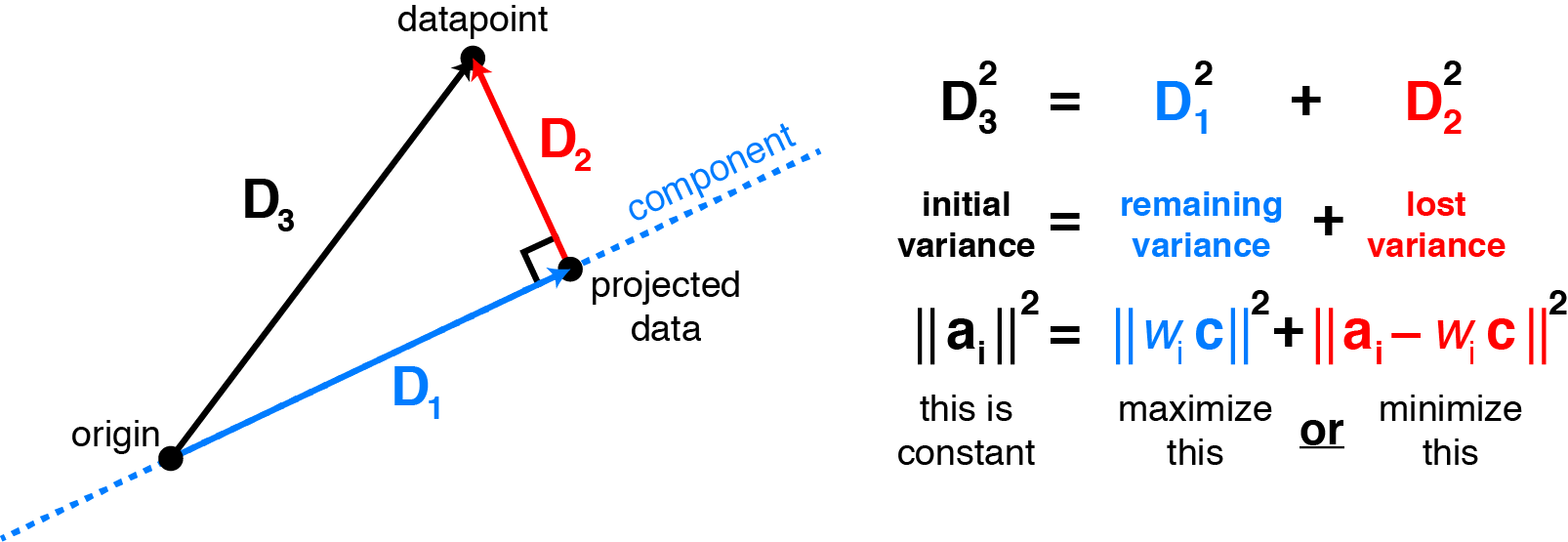
When we project the data onto some vector, we are essentially losing some of our original “variance”. When I say variance, I’m talking about the variance of our original data in terms of each variable. For example, if you decide to use p eigenvalues when your data has p columns, the sum of the eigenvalues will add up to the original “variance” of the data: $\sigma^2_1 + \sigma^2_2 + … + \sigma^2_p = {\lambda}_1 + {\lambda}_2 + … + {\lambda}_p$. It’s not the covariance matrix we are preserving essentially. Remember, the eigenvectors associated with the eigenvalue serve as the principal axes. Originally, the data is on the cartesian plane with the x and y axes for our 2d example. Now, we are going from 2d into 1d by projecting our data onto a line. This line has a direction associated with the largest eigenvalue of the covariance matrix of our data. That is what we call the eigenvector and this eigenvector serves as a “principal axis” now. It’s like we are going from one plane to another. The eigenvectors can be considered axes because the covariance matrix is a special type of matrix called a symmetric matrix. Symmetric matrices have eigenvectors that are orthogonal to one another. I know you shouldn’t take my word for it so here is a reference:
https://math.libretexts.org/Bookshelves/Linear_Algebra/A_First_Course_in_Linear_Algebra_(Kuttler) /07%3A_Spectral_Theory/7.04%3A_Orthogonality#:~: text=where%20D%20is%20a%20diagonal,is%20in%20fact%20orthogonally%20diagonalizable.
Hopefully, this helped a little when it comes to understanding PCA if you felt a little confused when first learning it. I know it’s not very mathematically sound so please do some more research on your own in regards to the proofs and such. Thanks for your time!
References
(Warning: Clicking the links will auto-download a pdf!)
- Proofs:
https://www.stat.cmu.edu/~cshalizi/uADA/12/lectures/ch18.pdf
- Visualizing PCA
https://alexhwilliams.info/itsneuronalblog/2016/03/27/pca/
- Visualizing PCA/Proof
https://web.lums.edu.pk/~imdad/pdfs/CS5312_Notes/CS5312_Notes-16-PCA.pdf